MNE-Python: KIT Attention Task Analysis (alpha lateralisation, raw vs CALM)
Lead authors: Hadi Zaatiti hadi.zaatiti@nyu.edu, Karima Raafat karima.raafat@nyu.edu
MNE-Python counterpart of the FieldTrip notebook Fieldtrip: KIT Attention Task Analysis, extended with the analysis of the EEG paper the task is modelled on:
Worden MS, Foxe JJ, Wang N, Simpson GV (2000). Anticipatory biasing of visuospatial attention indexed by retinotopically specific alpha-band electroencephalography increases over occipital cortex. J Neurosci 20(6):RC63.
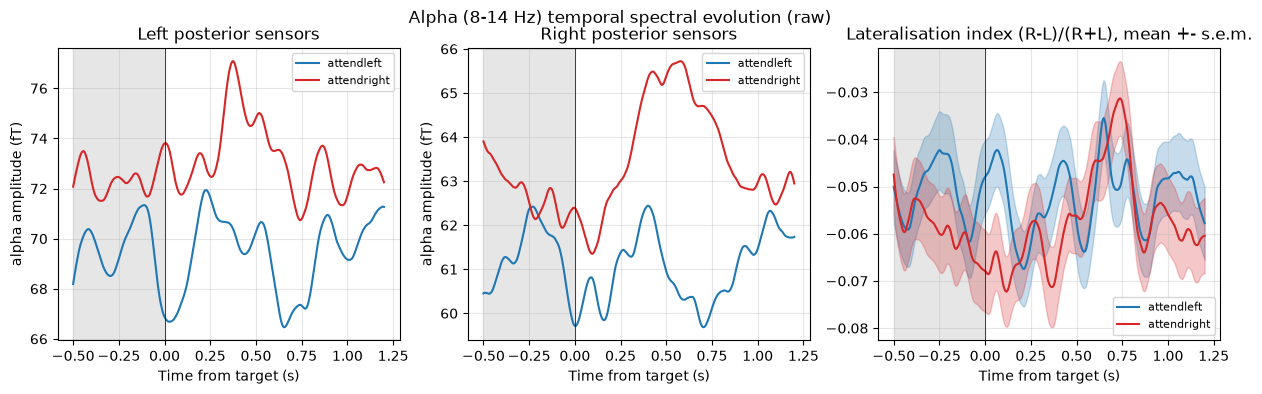
Prediction. Before a target appears, alpha-band (8-14 Hz) amplitude is higher over the hemisphere ipsilateral to the attended side and lower over the contralateral hemisphere. With the lateralisation index LI = (R - L) / (R + L) of posterior alpha amplitude, LI should be lower in the attend-left block than in the attend-right block.
Differences from the paper that matter. One subject; attention is cued once per 10-minute block (not trial by trial), and each block is a separate recording; there is no behavioural response; MEG axial gradiometers, sensor space only (no .mrk, so no head position and no source localisation). Every statistic below is therefore over trials of one subject, and the attention contrast is confounded with recording/block.
The whole analysis runs twice: on the original recordings and on the CALM noise-reduced ones.
Setup
Set the MEG_DATA environment variable to the Box MEG/Data folder.
[1]:
import os, json, warnings
from pathlib import Path
import numpy as np
import scipy.stats as ss
import matplotlib.pyplot as plt
import mne
mne.set_log_level("ERROR")
warnings.filterwarnings("ignore", category=RuntimeWarning)

MEG_DATA = Path(os.environ.get("MEG_DATA", Path.home() / "Box" / "MEG" / "Data"))
MEG_DIR = MEG_DATA / "attention-task" / "sub-001" / "meg"
OUT = Path(os.environ.get("ATTENTION_OUT", MEG_DATA / "attention-task" / "derivatives" / "mne_attention_task"))
OUT.mkdir(parents=True, exist_ok=True)

PROCS = {"raw": "", "CALM": "_proc-CALMnoisereduction"}
ACQS = ["attendleft", "attendright"]
# KIT trigger channels (0-based KIT index) -> (condition, event code)
TRIG = {224: ("AL_TR", 1), 225: ("AL_TL", 2), 226: ("AR_TR", 3), 227: ("AR_TL", 4)}
EVENT_ID = {name: code for name, code in TRIG.values()}
BLOCK_CODES = {"attendleft": [1, 2], "attendright": [3, 4]}
TMIN, TMAX = -0.5, 1.2            # same epoch as the FieldTrip notebook
BASELINE = (-0.2, 0.0)            # for the evoked fields only
PRE = (-0.5, 0.0)                 # anticipatory (pre-target) window for the alpha analysis
BANDS = {"theta": (4, 7), "alpha": (8, 14), "beta": (15, 25)}
DECIM = 4                         # 1000 Hz -> 250 Hz after filtering
SENSORS = {"MEG 147": "right posterior (AG147)", "MEG 183": "left posterior (AG183)"}
RNG = np.random.default_rng(0)

def con_path(acq, proc):
    return MEG_DIR / f"sub-001_task-attention_acq-{acq}{PROCS[proc]}_meg.con"

def savefig(name):
    plt.savefig(OUT / f"{name}.png", dpi=130, bbox_inches="tight"); plt.show(); plt.close()
Triggers
Four trial types, one KIT trigger channel each (224-227). The channels that are not used in a block carry only millivolt noise, so the FieldTrip “midpoint of min and max” threshold would turn that noise into thousands of events; a fixed 1 V threshold is used instead. A pulse that appears on more than one channel at the same time (one occurs 18 s before the attend-left block starts, on 225 and 226) is not a trial and is dropped.
[2]:
def find_events(raw, acq):
    chans = sorted(TRIG)
    hi = raw.get_data(picks=chans) > 1.0
    rows = []
    for k, ch in enumerate(chans):
        on = np.flatnonzero(hi[k, 1:] & ~hi[k, :-1]) + 1
        for s in on:
            if hi[:, max(s - 5, 0):s + 10].any(axis=1).sum() == 1:
                rows.append([s + raw.first_samp, 0, TRIG[ch][1]])
    ev = np.array(sorted(rows), int)
    return ev[np.isin(ev[:, 2], BLOCK_CODES[acq])]
Bad channels
A channel is bad if the log of its 1-40 Hz standard deviation is more than 4 robust z-scores from the median of all channels, in any of the four recordings. The union is removed everywhere so that raw and CALM are compared on identical sensors.
[3]:
def robust_z(x):
    med = np.median(x); return (x - med) / (1.4826 * np.median(np.abs(x - med)))

BADS = set(); noise_psd = {}
for proc in PROCS:
    for acq in ACQS:
        raw = mne.io.read_raw_kit(con_path(acq, proc), preload=True).pick("mag")
        psd = raw.compute_psd(method="welch", fmin=1, fmax=100, n_fft=4096)
        noise_psd[proc, acq] = (psd.freqs, psd.get_data())
        sd = raw.filter(1, 40).get_data().std(axis=1)
        bad = [raw.ch_names[i] for i in np.flatnonzero(np.abs(robust_z(np.log(sd))) > 4)]
        print(f"{proc:5s} {acq:11s} bad: {bad}")
        BADS |= set(bad)
        INFO = raw.info
        del raw
BADS = sorted(BADS); print("union of bad channels:", BADS)
raw   attendleft  bad: ['MEG 037', 'MEG 060', 'MEG 072', 'MEG 087', 'MEG 088', 'MEG 097', 'MEG 130', 'MEG 168', 'MEG 193']
raw   attendright bad: ['MEG 037', 'MEG 060', 'MEG 072', 'MEG 087', 'MEG 088', 'MEG 097', 'MEG 168']
CALM  attendleft  bad: ['MEG 123', 'MEG 193']
CALM  attendright bad: ['MEG 123', 'MEG 193']
union of bad channels: ['MEG 037', 'MEG 060', 'MEG 072', 'MEG 087', 'MEG 088', 'MEG 097', 'MEG 123', 'MEG 130', 'MEG 168', 'MEG 193']
Sensors and regions of interest
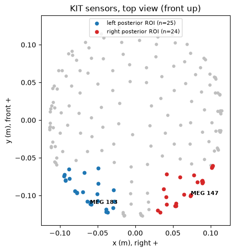
Without a head position we work in the helmet (device) frame: x to the right, y to the front. The left and right posterior regions are the sensors at the back of the helmet (y < -6 cm), at least 2 cm from the midline. MEG 147 and MEG 183 are the two sensors shown in the FieldTrip notebook (AG147, AG183).
[4]:
GOOD = [c for c in INFO.ch_names if c not in BADS]
info = mne.pick_info(INFO, mne.pick_channels(INFO.ch_names, GOOD, ordered=True))
pos = np.array([c["loc"][:3] for c in info["chs"]])
ROI_L = np.flatnonzero((pos[:, 1] < -0.06) & (pos[:, 0] < -0.02))
ROI_R = np.flatnonzero((pos[:, 1] < -0.06) & (pos[:, 0] > 0.02))
print(f"{len(GOOD)} good sensors; ROI left {len(ROI_L)}, right {len(ROI_R)}")

fig, ax = plt.subplots(figsize=(5.5, 5.5))
ax.scatter(pos[:, 0], pos[:, 1], s=14, c="0.75")
ax.scatter(*pos[ROI_L, :2].T, s=22, c="tab:blue", label=f"left posterior ROI (n={len(ROI_L)})")
ax.scatter(*pos[ROI_R, :2].T, s=22, c="tab:red", label=f"right posterior ROI (n={len(ROI_R)})")
for n in SENSORS:
    i = info.ch_names.index(n); ax.annotate(n, pos[i, :2], fontsize=8, weight="bold")
ax.set(title="KIT sensors, top view (front up)", xlabel="x (m), right +", ylabel="y (m), front +")
ax.set_aspect("equal"); ax.legend(fontsize=8, loc="upper center"); savefig("fig1_sensors_roi")
197 good sensors; ROI left 25, right 24
Preprocessing and epoching
For each recording: 1-40 Hz band-pass for the evoked fields; for each band (theta, alpha, beta) a band-pass followed by the Hilbert envelope, which is the “temporal spectral evolution” used by Worden et al. (band-pass, rectify, average). Epochs run from -0.5 to 1.2 s around target onset. Trials whose largest peak-to-peak amplitude is an outlier (robust z > 3.5 on the log scale) are rejected. Alpha epochs are not baseline-corrected: attention is sustained over the block, so the pre-target window is the effect, not a baseline.
[5]:
def process(acq, proc):
    raw = mne.io.read_raw_kit(con_path(acq, proc), preload=True)
    events = find_events(raw, acq)
    raw.pick(GOOD)
    eid = {k: v for k, v in EVENT_ID.items() if v in BLOCK_CODES[acq]}
    kw = dict(events=events, event_id=eid, tmin=TMIN, tmax=TMAX, decim=DECIM, preload=True)
    ep = mne.Epochs(raw.copy().filter(1, 40), baseline=None, **kw)
    ptp = np.ptp(ep.get_data(), axis=2).max(axis=1)
    keep = robust_z(np.log(ptp)) < 3.5
    env = {}
    for band, (lo, hi) in BANDS.items():
        e = mne.Epochs(raw.copy().filter(lo, hi).apply_hilbert(envelope=True), baseline=None, **kw)
        env[band] = e.get_data()[keep].astype(np.float32)
    ep = ep[np.flatnonzero(keep)]
    print(f"{proc:5s} {acq:11s} events {len(events)} kept {keep.sum()} "
          + str({k: len(ep[k]) for k in eid}))
    return dict(ep=ep, env=env, codes=ep.events[:, 2], n_events=len(events))

DATA = {proc: {acq: process(acq, proc) for acq in ACQS} for proc in PROCS}
times = DATA["raw"]["attendleft"]["ep"].times
pre = (times >= PRE[0]) & (times <= PRE[1])
raw   attendleft  events 462 kept 446 {'AL_TR': 224, 'AL_TL': 222}
raw   attendright events 462 kept 449 {'AR_TR': 221, 'AR_TL': 228}
CALM  attendleft  events 462 kept 459 {'AL_TR': 230, 'AL_TL': 229}
CALM  attendright events 462 kept 458 {'AR_TR': 228, 'AR_TL': 230}
Part 1 - the FieldTrip notebook in MNE
Evoked fields
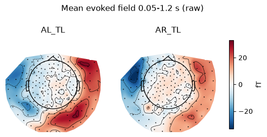
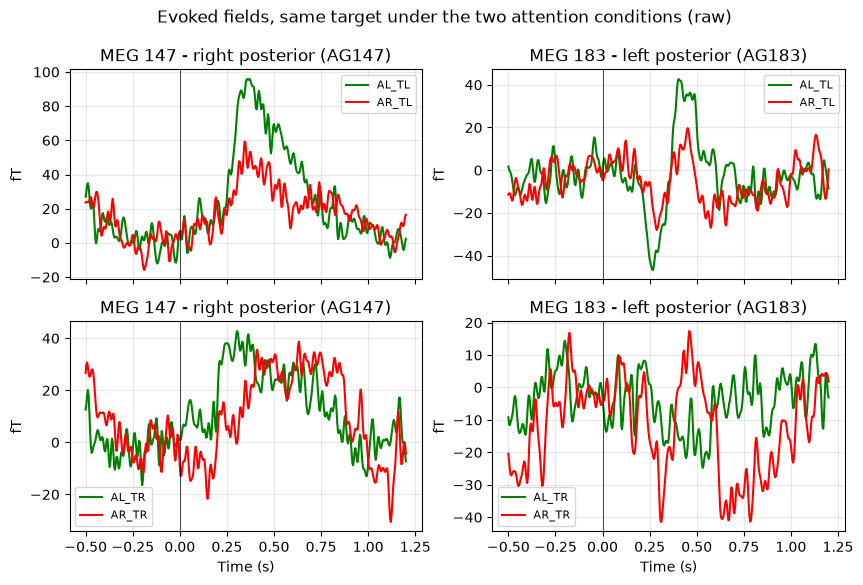
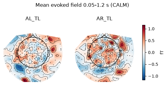
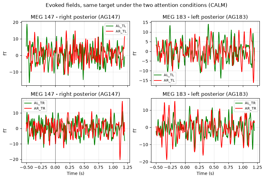
Averages per trial type (baseline -0.2 to 0 s), the mean field between 0.05 and 1.2 s for attend-left/target-left and attend-right/target-left, and the evoked responses at the two sensors for the same target under the two attention conditions.
[6]:
def evokeds(proc):
    out = {}
    for acq in ACQS:
        ep = DATA[proc][acq]["ep"]
        for k in ep.event_id:
            out[k] = ep[k].average().apply_baseline(BASELINE)
    return out

EVK = {proc: evokeds(proc) for proc in PROCS}
for proc in PROCS:
    fig, axes = plt.subplots(1, 2, figsize=(7, 3.4))
    win = (times >= 0.05) & (times <= 1.2)
    maps = [EVK[proc][k].data[:, win].mean(1) * 1e15 for k in ("AL_TL", "AR_TL")]
    vl = np.abs(maps).max()
    for ax, m, k in zip(axes, maps, ("AL_TL", "AR_TL")):
        im, _ = mne.viz.plot_topomap(m, info, axes=ax, show=False, vlim=(-vl, vl), cmap="RdBu_r")
        ax.set_title(k)
    fig.colorbar(im, ax=axes, shrink=0.7, label="fT")
    fig.suptitle(f"Mean evoked field 0.05-1.2 s ({proc})"); savefig(f"fig2_topo_evoked_{proc}")

    fig, axes = plt.subplots(2, 2, figsize=(10, 6), sharex=True)
    for r, (a, b) in enumerate([("AL_TL", "AR_TL"), ("AL_TR", "AR_TR")]):
        for c, s in enumerate(SENSORS):
            i = info.ch_names.index(s); ax = axes[r, c]
            ax.plot(times, EVK[proc][a].data[i] * 1e15, "g", label=a)
            ax.plot(times, EVK[proc][b].data[i] * 1e15, "r", label=b)
            ax.axvline(0, c="k", lw=0.5); ax.grid(alpha=0.3); ax.legend(fontsize=8)
            ax.set(title=f"{s} - {SENSORS[s]}", ylabel="fT")
    for ax in axes[1]: ax.set_xlabel("Time (s)")
    fig.suptitle(f"Evoked fields, same target under the two attention conditions ({proc})")
    savefig(f"fig3_erf_{proc}")
Alpha power over time (multitaper)
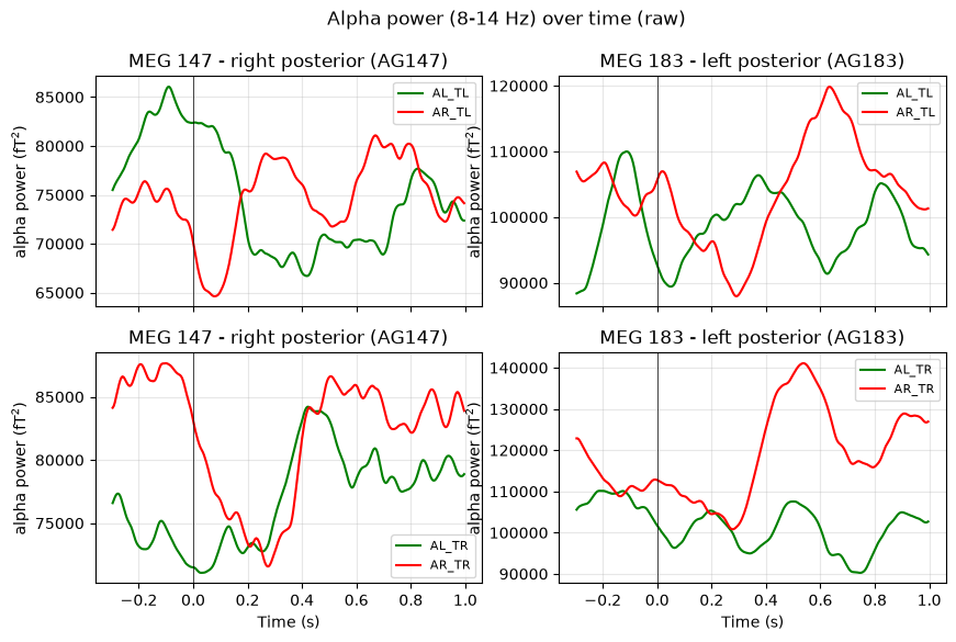
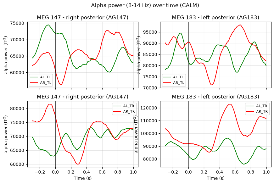
Same parameters as the FieldTrip cell (8-14 Hz, window of 3 cycles), with one difference: the FieldTrip notebook ran the time-frequency analysis on the trial average, which only keeps the phase-locked part. Here it is computed on single trials and then averaged, which is the induced plus evoked alpha power that the attention effect lives in. MNE needs a time-bandwidth product of at least 2, so the frequency smoothing is about +-3.3 Hz at 10 Hz instead of +-2.5 Hz.
[7]:
freqs = np.arange(8, 14.01, 0.5)
for proc in PROCS:
    tfr = {}
    for acq in ACQS:
        ep = DATA[proc][acq]["ep"]
        for k in ep.event_id:
            p = ep[k].compute_tfr("multitaper", freqs=freqs, n_cycles=3, time_bandwidth=2.0,
                                  picks=list(SENSORS), average=True)
            tfr[k] = p.data.mean(axis=1) * 1e30
    fig, axes = plt.subplots(2, 2, figsize=(10, 6), sharex=True)
    for r, (a, b) in enumerate([("AL_TL", "AR_TL"), ("AL_TR", "AR_TR")]):
        for c, s in enumerate(SENSORS):
            ax = axes[r, c]; sl = (times > -0.3) & (times < 1.0)
            ax.plot(times[sl], tfr[a][c][sl], "g", label=a); ax.plot(times[sl], tfr[b][c][sl], "r", label=b)
            ax.axvline(0, c="k", lw=0.5); ax.grid(alpha=0.3); ax.legend(fontsize=8)
            ax.set(title=f"{s} - {SENSORS[s]}", ylabel="alpha power (fT$^2$)")
    for ax in axes[1]: ax.set_xlabel("Time (s)")
    fig.suptitle(f"Alpha power (8-14 Hz) over time ({proc})"); savefig(f"fig4_alpha_tfr_{proc}")
Part 2 - the analysis of Worden et al. (2000)
Lateralisation index of pre-target alpha
Per trial, alpha amplitude is averaged over the pre-target window and over each posterior region, and LI = (R - L) / (R + L). Being a ratio, LI is insensitive to a global change of alpha between the two recordings. Trials are compared between blocks with a Welch t-test and a label permutation test. Successive trials are 1.3 s apart and not independent, so an adjusted t is also given that shrinks the sample size by the lag-1 autocorrelation r: n_eff = n (1 - r) / (1 + r).
[8]:
def li_of(a, axis_ch=1):
    L = a.take(ROI_L, axis=axis_ch).mean(axis_ch); R = a.take(ROI_R, axis=axis_ch).mean(axis_ch)
    return (R - L) / (R + L)

def compare(x_al, x_ar, n_perm=10000):
    """x_ar minus x_al; positive = the direction predicted by the paper."""
    diff = x_ar.mean() - x_al.mean()
    sp = np.sqrt((x_al.var(ddof=1) + x_ar.var(ddof=1)) / 2)
    t, p = ss.ttest_ind(x_ar, x_al, equal_var=False)
    allx = np.r_[x_al, x_ar]; n = len(x_al)
    perm = np.array([(lambda z: z[n:].mean() - z[:n].mean())(RNG.permutation(allx)) for _ in range(n_perm)])
    r1 = [np.corrcoef(x[:-1], x[1:])[0, 1] for x in (x_al, x_ar)]
    neff = [len(x) * (1 - r) / (1 + r) for x, r in zip((x_al, x_ar), r1)]
    se = np.sqrt(x_al.var(ddof=1) / neff[0] + x_ar.var(ddof=1) / neff[1])
    return dict(li_attend_left=float(x_al.mean()), li_attend_right=float(x_ar.mean()), diff=float(diff),
                cohen_d=float(diff / sp), t=float(t), p=float(p),
                p_perm=float((np.sum(np.abs(perm) >= abs(diff)) + 1) / (n_perm + 1)),
                lag1_autocorr=[float(r) for r in r1], t_adjusted=float(diff / se),
                p_adjusted=float(2 * ss.norm.sf(abs(diff / se))), n=[len(x_al), len(x_ar)])

RES = {proc: {} for proc in PROCS}
LI = {}
for proc in PROCS:
    for band in BANDS:
        li = [li_of(DATA[proc][acq]["env"][band][:, :, pre].mean(2)) for acq in ACQS]
        RES[proc][f"LI_{band}"] = compare(*li)
        if band == "alpha": LI[proc] = li
    r = RES[proc]["LI_alpha"]
    print(f"{proc:5s} alpha LI attend-left {r['li_attend_left']:+.4f}  attend-right {r['li_attend_right']:+.4f}  "
          f"diff {r['diff']:+.4f}  d={r['cohen_d']:+.2f}  t={r['t']:.2f} p={r['p']:.2g}  "
          f"perm p={r['p_perm']:.2g}  adjusted t={r['t_adjusted']:.2f} p={r['p_adjusted']:.2g}")
raw   alpha LI attend-left -0.0615  attend-right -0.0697  diff -0.0082  d=-0.09  t=-1.34 p=0.18  perm p=0.18  adjusted t=-1.37 p=0.17
CALM  alpha LI attend-left -0.0570  attend-right -0.0658  diff -0.0088  d=-0.10  t=-1.49 p=0.14  perm p=0.14  adjusted t=-1.55 p=0.12
Alpha time course in each hemisphere
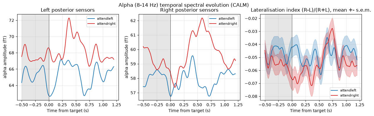
Alpha amplitude in the left and right posterior regions for the two attention blocks (all targets pooled), and the lateralisation index over time.
[9]:
for proc in PROCS:
    fig, axes = plt.subplots(1, 3, figsize=(15, 3.8))
    col = {"attendleft": "tab:blue", "attendright": "tab:red"}
    for acq in ACQS:
        e = DATA[proc][acq]["env"]["alpha"]
        for ax, roi, nm in zip(axes[:2], (ROI_L, ROI_R), ("Left", "Right")):
            ax.plot(times, e[:, roi].mean((0, 1)) * 1e15, c=col[acq], label=acq)
            ax.set(title=f"{nm} posterior sensors", xlabel="Time from target (s)", ylabel="alpha amplitude (fT)")
        l = li_of(e); m, s = l.mean(0), l.std(0, ddof=1) / np.sqrt(len(l))
        axes[2].plot(times, m, c=col[acq], label=acq); axes[2].fill_between(times, m - s, m + s, color=col[acq], alpha=0.25)
    axes[2].set(title="Lateralisation index (R-L)/(R+L), mean +- s.e.m.", xlabel="Time from target (s)")
    for ax in axes: ax.axvline(0, c="k", lw=0.5); ax.axvspan(*PRE, color="0.9", zorder=0); ax.legend(fontsize=8); ax.grid(alpha=0.3)
    fig.suptitle(f"Alpha (8-14 Hz) temporal spectral evolution ({proc})"); savefig(f"fig5_tse_{proc}")
Topography of the attention effect
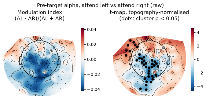
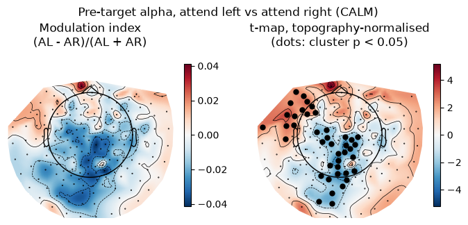
Left: modulation index (attend-left - attend-right) / (attend-left + attend-right) of mean pre-target alpha amplitude. Right: t-values of the same contrast after dividing every trial by its mean over sensors, which removes any global alpha difference between the two recordings and leaves the change in topography. Sensors in a significant cluster (cluster permutation test, 2000 permutations, two-sided) are marked. The paper predicts positive values on the left and negative on the right.
[10]:
adjacency, adj_names = mne.channels.find_ch_adjacency(INFO, "mag")
keep_adj = [adj_names.index(c) for c in info.ch_names]
adjacency = adjacency[keep_adj][:, keep_adj]
for proc in PROCS:
    A = [DATA[proc][acq]["env"]["alpha"][:, :, pre].mean(2).astype(float) for acq in ACQS]
    mi = (A[0].mean(0) - A[1].mean(0)) / (A[0].mean(0) + A[1].mean(0))
    X = [np.log(a) - np.log(a).mean(1, keepdims=True) for a in A]
    stat = lambda a, b: ss.ttest_ind(a, b, equal_var=False).statistic
    thr = ss.t.ppf(0.975, len(X[0]) + len(X[1]) - 2)
    T, clusters, pv, _ = mne.stats.permutation_cluster_test(X, stat_fun=stat, threshold=thr, tail=0,
                                                           adjacency=adjacency, n_permutations=2000, seed=0, out_type="mask")
    mask = np.zeros(len(T), bool); cl = []
    for c, p in zip(clusters, pv):
        if p < 0.05:
            mask |= c
            cl.append(dict(p=float(p), n_sensors=int(c.sum()), mean_t=float(T[c].mean()), mean_x_cm=float(pos[c, 0].mean() * 100),
                           mean_y_cm=float(pos[c, 1].mean() * 100)))
    RES[proc]["clusters"] = cl; RES[proc]["global_alpha_ratio_AL_over_AR"] = float(A[0].mean() / A[1].mean())
    RES[proc]["mi_left_roi"] = float(mi[ROI_L].mean()); RES[proc]["mi_right_roi"] = float(mi[ROI_R].mean())
    print(proc, "significant clusters:", cl)
    fig, axes = plt.subplots(1, 2, figsize=(8.5, 3.8))
    v = np.abs(mi).max(); im, _ = mne.viz.plot_topomap(mi, info, axes=axes[0], show=False, vlim=(-v, v), cmap="RdBu_r")
    axes[0].set_title("Modulation index\n(AL - AR)/(AL + AR)"); fig.colorbar(im, ax=axes[0], shrink=0.7)
    v = np.abs(T).max(); im, _ = mne.viz.plot_topomap(T, info, axes=axes[1], show=False, vlim=(-v, v), cmap="RdBu_r",
                                                      mask=mask, mask_params=dict(markersize=5, markerfacecolor="k"))
    axes[1].set_title("t-map, topography-normalised\n(dots: cluster p < 0.05)"); fig.colorbar(im, ax=axes[1], shrink=0.7)
    fig.suptitle(f"Pre-target alpha, attend left vs attend right ({proc})"); savefig(f"fig6_topo_attention_{proc}")
raw significant clusters: [{'p': 0.04, 'n_sensors': 8, 'mean_t': 2.6081473282831924, 'mean_x_cm': -9.5605625, 'mean_y_cm': 6.4826999999999995}, {'p': 0.0005, 'n_sensors': 30, 'mean_t': -2.670149192683234, 'mean_x_cm': -1.1898633333333333, 'mean_y_cm': -5.87243}]
CALM significant clusters: [{'p': 0.007, 'n_sensors': 14, 'mean_t': 2.446976504593615, 'mean_x_cm': -9.735778571428574, 'mean_y_cm': 5.261464285714287}, {'p': 0.0005, 'n_sensors': 27, 'mean_t': -2.5287982169016576, 'mean_x_cm': -0.30801481481481485, 'mean_y_cm': -6.680237037037037}]
Is the block difference larger than the drift within a block?
The two attention conditions are two separate 10-minute recordings, so anything that changes slowly (head position, vigilance) is confounded with attention. The running lateralisation index across trials shows how much LI moves within a block, and the split-half values give the size of that drift to compare with the between-block difference.
[11]:
for proc in PROCS:
    fig, axes = plt.subplots(1, 2, figsize=(13, 3.8), gridspec_kw=dict(width_ratios=[2.2, 1]))
    k = 40; off = 0; halves = {}
    for acq, c in zip(ACQS, ("tab:blue", "tab:red")):
        x = LI[proc][ACQS.index(acq)]
        run = np.convolve(x, np.ones(k) / k, mode="valid")
        axes[0].plot(off + np.arange(len(x)), x, ".", c=c, ms=2, alpha=0.35)
        axes[0].plot(off + k // 2 + np.arange(len(run)), run, c=c, lw=2, label=f"{acq} (running mean, {k} trials)")
        axes[1].hist(x, bins=30, color=c, alpha=0.5, label=acq)
        h = len(x) // 2; halves[acq] = [float(x[:h].mean()), float(x[h:].mean())]
        off += len(x) + 20
    RES[proc]["LI_alpha_split_half"] = halves
    RES[proc]["within_block_drift"] = float(np.mean([abs(v[1] - v[0]) for v in halves.values()]))
    axes[0].set(xlabel="Trial (attend-left recording, then attend-right recording)", ylabel="LI (R-L)/(R+L)")
    axes[0].legend(fontsize=8); axes[0].grid(alpha=0.3); axes[1].set(xlabel="LI"); axes[1].legend(fontsize=8)
    fig.suptitle(f"Pre-target alpha lateralisation per trial ({proc})"); savefig(f"fig7_li_trials_{proc}")
    print(proc, "split-half LI:", halves, " between-block diff:", round(RES[proc]["LI_alpha"]["diff"], 4))
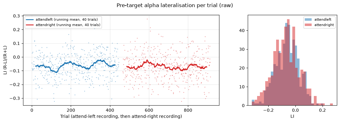
raw split-half LI: {'attendleft': [-0.06750579923391342, -0.0555427260696888], 'attendright': [-0.062262050807476044, -0.07706770300865173]} between-block diff: -0.0082
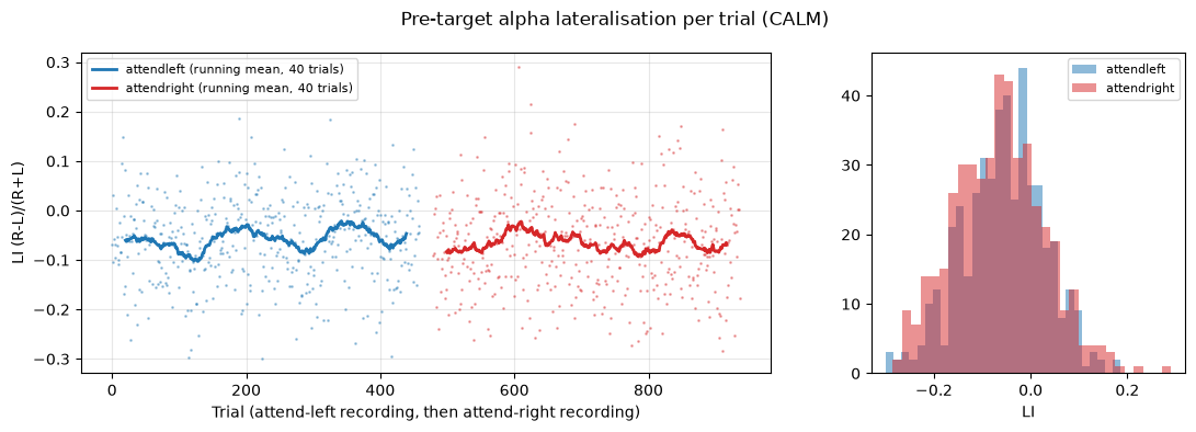
CALM split-half LI: {'attendleft': [-0.060856349766254425, -0.05313107743859291], 'attendright': [-0.060564324259757996, -0.07097858935594559]} between-block diff: -0.0088
Is the effect specific to alpha?
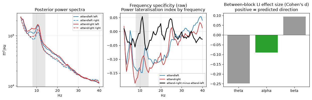
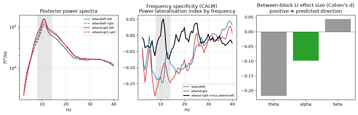
The lateralisation index as a function of frequency (multitaper spectra of the whole epoch) for the two blocks, and the between-block effect size for theta, alpha and beta envelopes. An effect of attention on alpha should peak in the alpha band; a geometric difference between the two recordings (head position) would shift LI at all frequencies.
[12]:
for proc in PROCS:
    fig, axes = plt.subplots(1, 3, figsize=(15, 3.8)); spec = {}
    for acq, c in zip(ACQS, ("tab:blue", "tab:red")):
        d = DATA[proc][acq]["ep"].get_data()
        psd, f = mne.time_frequency.psd_array_multitaper(d, 1000 / DECIM, fmin=2, fmax=40, bandwidth=2.0, verbose=False)
        L, R = psd[:, ROI_L].mean((0, 1)), psd[:, ROI_R].mean((0, 1)); spec[acq] = (R - L) / (R + L)
        axes[0].semilogy(f, L * 1e30, c=c, ls="-", label=f"{acq} left"); axes[0].semilogy(f, R * 1e30, c=c, ls="--", label=f"{acq} right")
        axes[1].plot(f, spec[acq], c=c, label=acq)
    axes[1].plot(f, spec["attendright"] - spec["attendleft"], "k", lw=2, label="attend-right minus attend-left")
    axes[0].set(title="Posterior power spectra", xlabel="Hz", ylabel="fT$^2$/Hz"); axes[1].set(title="Power lateralisation index by frequency", xlabel="Hz")
    for ax in axes[:2]: ax.axvspan(8, 14, color="0.9", zorder=0); ax.legend(fontsize=7); ax.grid(alpha=0.3)
    d = [RES[proc][f"LI_{b}"]["cohen_d"] for b in BANDS]
    axes[2].bar(list(BANDS), d, color=["0.6", "tab:green", "0.6"]); axes[2].axhline(0, c="k", lw=0.5)
    axes[2].set(title="Between-block LI effect size (Cohen's d)\npositive = predicted direction")
    a = (f >= 8) & (f <= 14); dd = spec["attendright"] - spec["attendleft"]
    RES[proc]["li_spectrum_diff"] = dict(alpha=float(dd[a].mean()), theta=float(dd[(f >= 4) & (f <= 7)].mean()),
                                         beta=float(dd[(f >= 15) & (f <= 25)].mean()), gamma_30_40=float(dd[f >= 30].mean()))
    fig.suptitle(f"Frequency specificity ({proc})"); savefig(f"fig8_band_specificity_{proc}")
Part 3 - raw versus CALM
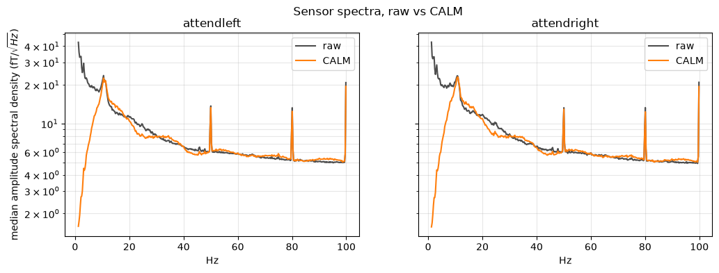
Sensor noise spectra before and after CALM, and the main numbers side by side.
[13]:
fig, axes = plt.subplots(1, 2, figsize=(12, 3.8), sharey=True)
gi = [INFO.ch_names.index(c) for c in GOOD]
for ax, acq in zip(axes, ACQS):
    for proc, c in zip(PROCS, ("0.3", "tab:orange")):
        f, p = noise_psd[proc, acq]
        ax.semilogy(f, np.sqrt(np.median(p[gi], 0)) * 1e15, c=c, label=proc)
    ax.set(title=acq, xlabel="Hz"); ax.grid(alpha=0.3, which="both"); ax.legend()
axes[0].set_ylabel("median amplitude spectral density (fT/$\\sqrt{Hz}$)")
fig.suptitle("Sensor spectra, raw vs CALM"); savefig("fig9_psd_raw_vs_calm")

for proc in PROCS:
    for acq in ACQS:
        f, p = noise_psd[proc, acq]; m = np.median(p[gi], 0)
        band = lambda lo, hi: float(np.sqrt(m[(f >= lo) & (f <= hi)].mean()) * 1e15)
        RES[proc][f"asd_fT_{acq}"] = {"1-4Hz": band(1, 4), "8-14Hz": band(8, 14), "20-40Hz": band(20, 40), "49-51Hz": band(49, 51)}
    RES[proc]["trials_kept"] = {acq: [int(len(DATA[proc][acq]["codes"])), int(DATA[proc][acq]["n_events"])] for acq in ACQS}
    e = EVK[proc]
    RES[proc]["erf_peak_fT"] = {k: float(np.abs(e[k].data[:, (times > 0.05) & (times < 0.4)]).max() * 1e15) for k in e}
    RES[proc]["erf_prestim_rms_fT"] = {k: float(e[k].data[:, times < 0].std() * 1e15) for k in e}
RES["bad_channels"] = BADS; RES["roi"] = dict(left=[info.ch_names[i] for i in ROI_L], right=[info.ch_names[i] for i in ROI_R])
json.dump(RES, open(OUT / "results.json", "w"), indent=1)

rows = [("alpha LI, attend left", lambda r: f"{r['LI_alpha']['li_attend_left']:+.4f}"),
        ("alpha LI, attend right", lambda r: f"{r['LI_alpha']['li_attend_right']:+.4f}"),
        ("difference (predicted > 0)", lambda r: f"{r['LI_alpha']['diff']:+.4f}"),
        ("Cohen's d", lambda r: f"{r['LI_alpha']['cohen_d']:+.2f}"),
        ("Welch t / p", lambda r: f"{r['LI_alpha']['t']:.2f} / {r['LI_alpha']['p']:.2g}"),
        ("permutation p", lambda r: f"{r['LI_alpha']['p_perm']:.2g}"),
        ("autocorrelation-adjusted t / p", lambda r: f"{r['LI_alpha']['t_adjusted']:.2f} / {r['LI_alpha']['p_adjusted']:.2g}"),
        ("within-block split-half drift", lambda r: f"{r['within_block_drift']:.4f}"),
        ("d theta / beta", lambda r: f"{r['LI_theta']['cohen_d']:+.2f} / {r['LI_beta']['cohen_d']:+.2f}"),
        ("significant sensor clusters", lambda r: str(len(r['clusters']))),
        ("trials kept (AL, AR)", lambda r: f"{r['trials_kept']['attendleft'][0]}, {r['trials_kept']['attendright'][0]}")]
print(f"{'':34s}{'raw':>18s}{'CALM':>18s}")
for name, fn in rows:
    print(f"{name:34s}{fn(RES['raw']):>18s}{fn(RES['CALM']):>18s}")
                                                 raw              CALM
alpha LI, attend left                        -0.0615           -0.0570
alpha LI, attend right                       -0.0697           -0.0658
difference (predicted > 0)                   -0.0082           -0.0088
Cohen's d                                      -0.09             -0.10
Welch t / p                             -1.34 / 0.18      -1.49 / 0.14
permutation p                                   0.18              0.14
autocorrelation-adjusted t / p          -1.37 / 0.17      -1.55 / 0.12
within-block split-half drift                 0.0134            0.0091
d theta / beta                         -0.25 / +0.09     -0.22 / +0.04
significant sensor clusters                        2                 2
trials kept (AL, AR)                        446, 449          459, 458
Results for sub-001 (run of 2026-11-13)
The lateralisation reported by Worden et al. (2000) is not reproduced in this recording.
Pre-target alpha LI is -0.057 (attend left) and -0.066 (attend right) with CALM; the difference, -0.009, is in the direction opposite to the prediction and not significant (Cohen’s d = -0.10, permutation p = 0.14). Without CALM: -0.008, d = -0.09, p = 0.18.
LI drifts by about 0.01 between the two halves of a single block, as much as the difference between blocks, so the block contrast cannot be separated from slow drift.
The sensor map of attend-left minus attend-right is not a left/right flip over posterior sensors: it is a midline posterior decrease plus a left-frontal increase (both clusters p < 0.05). With two separate recordings and no head position, a small change of head position or vigilance explains this at least as well as attention does.
The theta-band LI differs between blocks more than alpha does (d = -0.22), which also points to a non-specific difference between the recordings.
Exploratory, not tested: the LI spectrum shows a narrow difference in the predicted direction at the alpha peak (10-11 Hz) and the opposite sign at 12-14 Hz, which cancel in the 8-14 Hz band.
No target-evoked field is visible at the two sensors: the target is nearly isoluminant by design.
CALM versus raw. CALM lowers the median sensor noise at 1-4 Hz from about 30 to 3.4 fT/sqrt(Hz), leaves 8-14 Hz almost unchanged (18 to 17), halves the pre-stimulus noise of the evoked fields and rescues about 10 trials per block from rejection. The attention result is the same with and without it.
What would make the test conclusive. Cue attention trial by trial (or alternate short blocks within one recording), add a behavioural response at the attended location so that attention is actually engaged and can be verified, record the .mrk head position and eye position, and collect a group of subjects.